4.3 Stanley

The Stanley controller for path tracking explained, with its equations and a Python simulation. The Stanley controller steers a vehicle along a reference course by looking at two errors at the front axle: how far the axle is from the course, and how much the vehicle’s heading differs from the course’s direction. After this section, you can compute its steering angle by hand and change its gain in the simulation.

Problem and intuition

A path tracking controller has to decide the steering angle at every time step so that the vehicle follows a given course. The Stanley controller was used by Stanford’s car “Stanley”, which won the DARPA Grand Challenge in 2005 [1].

It combines two simple ideas:

• Align with the course. If the vehicle points in a different direction from the course, turn the wheels by that difference.

• Steer back toward the course. If the front axle is off to one side, turn toward the course. The farther away, the more you turn, but the faster you drive, the less you turn, so the vehicle doesn’t swerve at high speed.

Both are measured at the front axle, because the front wheels are the ones that steer.

Run it from the repository root: python src/simulations/path_tracking/stanley_path_tracking/stanley_path_tracking.py (code on GitHub)

Theory

The symbols follow Notation and Units.

Front axle position. The vehicle’s state \((x, y, \theta, v)\) is given at the rear axle. The front axle is the wheelbase \(L\) ahead along the heading:

\[ x_f = x + L\cos\theta, \qquad y_f = y + L\sin\theta \tag{1} \]

Errors. Let \((x_r, y_r, \theta_r)\) be the point on the course nearest to the front axle and the course’s yaw there. The heading error \(\theta_e\) and the lateral error \(e\) are

\[ \theta_e = \theta - \theta_r, \qquad e = -\sin\theta\,(x_f - x_r) + \cos\theta\,(y_f - y_r) \tag{2} \]

\(e\) is the front axle’s offset from the course point, measured along the vehicle’s left direction: it is positive when the axle is on the left of the course.

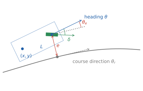
The errors at the front axle and the steering angle of equation (3). Here the front axle is on the left of the course and the vehicle points to the left of it, so both \(e\) and \(\theta_e\) are positive and \(\delta\) turns right.

Steering law. The steering angle \(\delta\) (positive to the left) is

\[ \delta = -\left(\theta_e + \arctan\frac{k\,e}{v}\right) \tag{3} \]

• The first term turns the wheels back by the heading error. If the vehicle points 0.1 rad to the left of the course, the wheels turn 0.1 rad to the right.

• The second term steers toward the course. For a small offset, \(\arctan(k e / v) \approx k e / v\): the correction grows with the offset and shrinks with the speed. For a large offset it saturates at \(\pi/2\), so the vehicle heads straight for the course instead of turning more and more.

The minus sign comes from the sign convention of (2): both errors are positive when the vehicle is to the left of or turned to the left of the course, and the correction turns right. Snider [2] defines the errors with the opposite signs and writes the same law without the minus sign.

Yaw rate. The vehicle model of this project takes a yaw rate as its input, so the steering angle is turned into a yaw rate with the kinematic bicycle model:

\[ \omega = \frac{v \tan\delta}{L} \tag{4} \]

Speed. The speed follows the course’s target speed \(v_r\) with a proportional controller, \(a = k_v (v_r - v)\).

Algorithm

At every time step, given the state (x, y, theta, v) at the rear axle:
1. Compute the front axle position with (1)
2. Find the course point nearest to the front axle
3. Compute the heading error and the lateral error with (2)
4. Compute the steering angle with (3), using 0 for the arctan term when v = 0
5. Compute the yaw rate with (4), and the acceleration from the target speed

Limits

• Low speed. \(k e / v\) grows without bound as \(v \to 0\), so the steering can jump at very low speed. The original paper adds a softening constant, \(\arctan(k e / (k_s + v))\) [1]. This implementation has no softening constant, and only skips the term when \(v = 0\).

• Gain tuning. A small \(k\) returns to the course slowly. A large \(k\) returns quickly but can oscillate.

• Lateral error in the vehicle’s frame. (2) measures the offset along the vehicle’s left direction, not perpendicular to the course. The two agree when the heading error is small, which is the normal case while tracking.

• Kinematic model only. The law ignores tire slip and actuator delay. The paper adds terms for them at high speed [1].

Where the equations live in the code

The controller is StanleyController in src/components/control/stanley/stanley_controller.py. Its update() runs the five steps of the algorithm:

    def update(self, state, time_s):
        """
        Function to update data for path tracking
        state: Vehicle's state object
        time_s: Simulation interval time[sec]
        """

        if not self.course: return

        front_axle_state = self._calculate_front_axle_state(state)

        self._calculate_target_course_index(front_axle_state)

        self._decide_target_speed_mps()

        self._calculate_target_acceleration_mps2(front_axle_state)

        _, error_lat_m, error_yaw_rad = self._calculate_tracking_error(front_axle_state)

        self._calculate_control_input(front_axle_state, error_lat_m, error_yaw_rad)

Equation (1), the front axle position:

    def _calculate_front_axle_state(self, state):
        """
        Private function to calculate state of front axle
        state: State object of vehicle's rear axle
        Return state object of vehicle's front axle
        """

        # current rear axle position and pose
        curr_rear_x = state.get_x_m()
        curr_rear_y = state.get_y_m()
        curr_yaw = state.get_yaw_rad()
        curr_spd = state.get_speed_mps()

        # calculate front axle position
        curr_front_x = curr_rear_x + self.WHEEL_BASE_M * cos(curr_yaw)
        curr_front_y = curr_rear_y + self.WHEEL_BASE_M * sin(curr_yaw)
        curr_front_state = State(curr_front_x, curr_front_y, curr_yaw, curr_spd)

        return curr_front_state

Equation (2) is computed by the course, which knows the target point. error_yaw_rad is \(\theta_e\) and error_lat_m is \(e\):

    def calculate_lonlat_error(self, state, point_index):
        """
        Function to calculate longitudinal/lateral/yaw angle error against course
        state: Vehicle's state object
        point_index: index of point on course
        """
        
        error_x_m = state.get_x_m() - self.x_array[point_index]
        error_y_m = state.get_y_m() - self.y_array[point_index]

        current_yaw_rad = state.get_yaw_rad()
        error_yaw_rad = pi_to_pi(current_yaw_rad - self.yaw_array[point_index])

        error_lon_m = cos(current_yaw_rad) * error_x_m + sin(current_yaw_rad) * error_y_m
        error_lat_m = -sin(current_yaw_rad) * error_x_m + cos(current_yaw_rad) * error_y_m

        return error_lon_m, error_lat_m, error_yaw_rad

Equations (3) and (4). CONTROL_GAIN is \(k\), and atan2(k e, v) equals \(\arctan(k e / v)\) for \(v > 0\):

    def _calculate_control_input(self, state, error_lat_m, error_yaw_rad):
        """
        Private function to calculate yaw rate input
        state: State object of vehicle's front axle
        error_lat_m: Lateral error against reference course[m]
        error_yaw_rad: Yaw angle error against reference course[rad]
        """

        # calculate steering angle input
        curr_spd = state.get_speed_mps()
        if abs(curr_spd) != 0.0:
            error_steer_rad = atan2(self.CONTROL_GAIN * error_lat_m, curr_spd)
        else:
            error_steer_rad = 0.0
        self.target_steer_rad = -1 * (error_steer_rad + error_yaw_rad)

        # calculate yaw rate input
        self.target_yaw_rate_rps = curr_spd * tan(self.target_steer_rad) / self.WHEEL_BASE_M

Experiments

Run the simulation src/simulations/path_tracking/stanley_path_tracking/stanley_path_tracking.py, and change self.CONTROL_GAIN in the constructor of StanleyController (0.5 by default):

• With 0.1, the vehicle comes back to the course slowly after the curves.

• With 2.0, it comes back quickly. Watch whether it starts to weave around the course.

Exercises

1. A vehicle drives at \(v = 5\) m/s with its front axle \(e = 1\) m to the left of a straight course, pointing along the course (\(\theta_e = 0\)). With \(k = 0.5\), compute \(\delta\) with (3). Then compute it for \(v = 1\) m/s. Why does the vehicle steer harder at the lower speed?

2. Add the softening constant \(k_s\) of the original paper to _calculate_control_input(), and check how the steering behaves when the simulation starts from rest.

3. Run the Pure Pursuit simulation (src/simulations/path_tracking/pure_pursuit_path_tracking) on the same course, and compare how closely the two controllers follow the curves.

References

1. G. M. Hoffmann, C. J. Tomlin, M. Montemerlo and S. Thrun, “Autonomous Automobile Trajectory Tracking for Off-Road Driving: Controller Design, Experimental Validation and Racing”, American Control Conference, 2007. PDF

2. J. M. Snider, “Automatic Steering Methods for Autonomous Automobile Path Tracking”, Technical Report CMU-RI-TR-09-08, Carnegie Mellon University, 2009. PDF